Large dataset
Note
We define a dataset as large if it is intended for use with microbetagDB and contains several thousand taxa (sequence IDs).
While the number of samples also influences microbetag’s runtime, its impact is significantly smaller.
If you want to annotate a dataset of any size using your own genomes, bins, or MAGs, follow the corresponding tutorial here.
In case of large datasets, microbetag full on-the-fly run is probably not an option,
even if you do run the preprocessing step.
For example, imagine you have a 16S rRNA marker-gene dataset and a couple of hundreds of samples.
Based on the microbetag_prep tutorial, you have taxonomically annotated them with the
GTDB-oriented 16S reference database, and you built a co-occurrence network using FlashWeave.
Now, let’s say you wish to perform network clustering on your network.
Asking for this on the on-the-fly version of microbetag will lead to a RuntimeError and your session will probably fail.
Important
When working with large datasets, it is strongly suggested you run as many steps as possible locally.
In its current version, the microbetag stand-alone tool does not support making API queries on microbetagDB
but this is on
top of our to-do list.
In this tutorial, we show how we handled such a large dataset.
16S rRNA data of hundreds of sub-gingival plaque samples from a Qiita project
From the record of the Human Microbiome Project (HMP) on
Qiita,
we first got the .biom of the study, and
using the
biom tols,
we converted the .biom file to a .txt
biom convert -i otu_table.biom -o hmp_otu_table.txt --to-tsv --header-key taxonomy
With the
get_biom.R
script of ours,
we were able to only collect subgingival plaque samples and get rid of zero abundance taxa,
building the
Subgingival_plaque.txt file.
In Qiita, the first column corresponds to Silva sequence identifiers in which the OTUs of the study were mapped against.
Since we cannot get directly the OTUs of the study, we used those identifiers, and with the Silva_119_release.zip
from the Silva archive,
we got their Silva closest ones.
This way, we ended up with an abundance table which in its last column had the Silva sequence instead of the taxonomy
(Subgingival_plaque_Silva_seq.csv).
Note
The code for this part is not included since this is beyond the scope of this tutorial.
The point of this step is that we started with a taxonomy table which had a rather old Silva version
and we built an abundance table with the corresponding sequences instead of the taxonomies,
in order to use the microbetag_prep tool.
In case you have your own OTUs/ASVs, you just need to use the abundance table with those along with the microbetag_prep tool.
Using the Subgingival_plaque_taxonomy_Silva_seq.csv,
we used the Docker microbetag_prep tool to get
a GTDB-based taxonomy assignment and a FlashWeave network.
To this end, we first created a folder called subgingival_plaque where we moved the
Subgingival_plaque_taxonomy_Silva_seq.csv file.
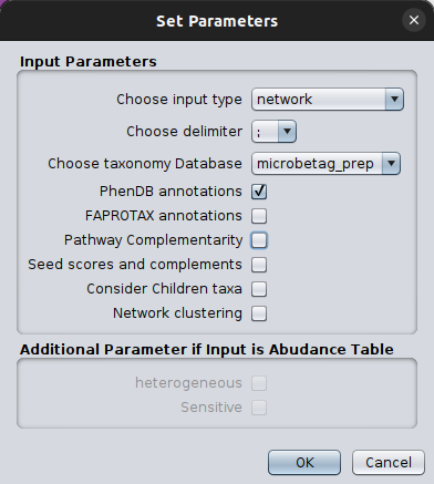
We then downloaded the config.yml file for the microbetag_prep tool,
and we set its parameters accordingly.
In this case, we set the sensitive parameter as false, since the number of taxa present would lead to
a vast number of associations.
The heterogeneous parameter was also set to false.
We then ran:
docker run --rm -it --entrypoint /bin/bash -v ./subgingival_plaque:/media hariszaf/microbetag_prep:v1.0.1
This entered us on a container where our input data would be under /media.
    root@50a101bce75f:/pre_microbetag# ls /media/
    Subgingival_plaque_Silva_seq.csv  config.yml
we then ran the microbetag_prep
root@9741096f8593:/pre_microbetag# python3 prep.py /media/config.yml
which resulted in the prep_output folder, in the mounted /media folder:
    root@9741096f8593:/pre_microbetag# ls /media/prep_output
    GTDB_tax_assigned_abundance_table.tsv  network_output.edgelist
Attention
CONFIGURATION FILE VERSIONING
Make sure that you always use the configuration file version that matches the tool version you are using.
Thus, microbetag_prep returned
GTDB_tax_assigned_abundance_table.tsv
that keeps the same sequence identifiers as the original, but now
the taxonomy has been replaced and instead of the Silva one, we have the GTDB.
Also, the network_output.edgelist
is the result of FlashWeave.
Up to this point, we actually run the microbetag_prep tutorial.
So now, as in the preparation tutorial, we can use those two files with the on-the-fly version.
Only this time, we can combine them with the stand-alone tool and/or the microbetag API.
So next, what we did was to run the on-the-fly version asking only for the FAPROTAX and the phenDB-like annotations, i.e. the node-level annotations.
Hint
Since we already have a network and our taxonomies in microbetag’s prefered scheme,
node-level annotations scale well on the on-the-fly version of microbetag! 🚀
However, you may also go for a step-by-step approach, retrieving first a FAPROTAX-annotated network and then, itse phenDB-like traits.
Load base network - edgelist
From File > Import > Network from file we loaded the network_output.edgelist as it was returned
by the microbetag_prep tool.
We then loaded our updated taxonomy table (GTDB_tax_assigned_abundance_table) on MGG by clicking
Apps > MGG > Import Data > Import Abundance Data.
We also loaded the already displayed on the main panel network of ours, on MGG, by clicking
Apps > MGG > Import Data > Import Current Network.
We then performed a first round of microbetag annotation asking only for the FAPROTAX step

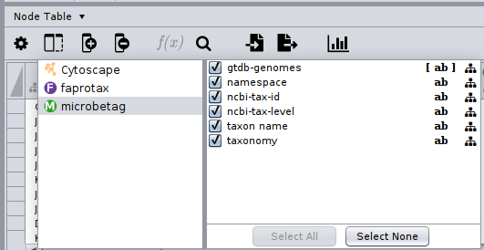
After a few seconds we got back a FAPROTAX annotated network; by clicking on the Show Columns... button of the Nodes table,
we may see what are the namespaces of the columns of our network:
We then used the FAPROTAX annotated network as input for a second round of microbetag annotation,
this time requiring only the phenDB step.
and after a couple of seconds we got back a network with both the phenDB-like annotations and the previous from FAPROTAX!

Now, we wanted to cluster our network using the manta algorithm that microbetag also makes use of.
We could do this either by installing manta and run it independently, or you can use it through the stand-alone tool.
Using the microbetag wrapping functions we wrote the manta_large_dataset.py
to run manta.
As you can see, this script makes use of the initial network.edgelist and is independent of the annotation steps
we performed above.
After a couple of minutes (~15’, depends on your computing system),
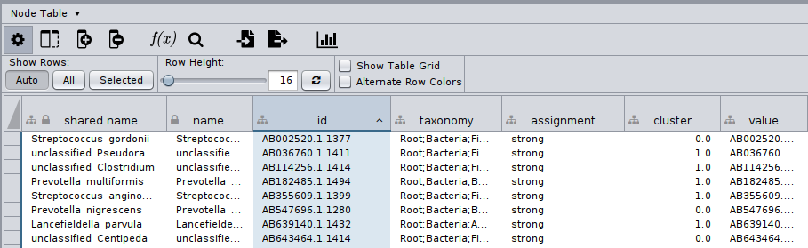
we got the manta_annotated.cyjs,
a network in CYJS format carrying only the initial nodes and eges, and two new columns, one called cluster with the number
of the assigned cluster to each node, and another called assignement with a characterization of the assignment
either as strong or week.
Note
The manta_basenet.cyjs that was also returned, it is required from manta to run and it is just
the initially provided network but in a CYJS format.
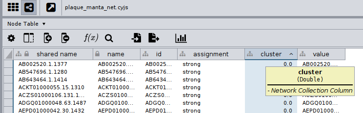
Now, we can load on Cytoscape the manta_annotated.cyjs clustered network, the same way we did before for the initial network.
The node table of this would look like:
Finally, we can bring our clusters together with our node annotations by importing a table!
To do this, we had to first export the manta annotated node table
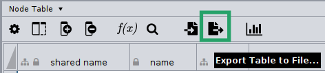
You can find the exported table called manta_annotated.node.csv
here
Hint
On the exported .csv with the cluster column, make sure you convert the column to integer.
microbetag expects the microbetag::cluster to be integer, and clustering algorithms may return clusters as float!
An easy way to do this is by using the Function Builder on the Node table.
First, click on the Create a New Column .. option and set it as Integer.
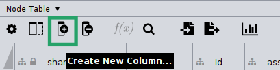
Then, make sure you call the new column microbetag::cluster; this is required for the enrichment analysis to run.
After you create the new column, click on it on the Nodes table, and then click the Function Builder button.
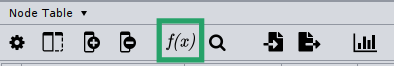
Now, you are about to describe how your new column should be filled in.
So, we will ask for the absolute value of the cluster column of ours.
In this case, this is the manta outcome, but it could be from any network clustering algorithm.
This column may be called whatever.
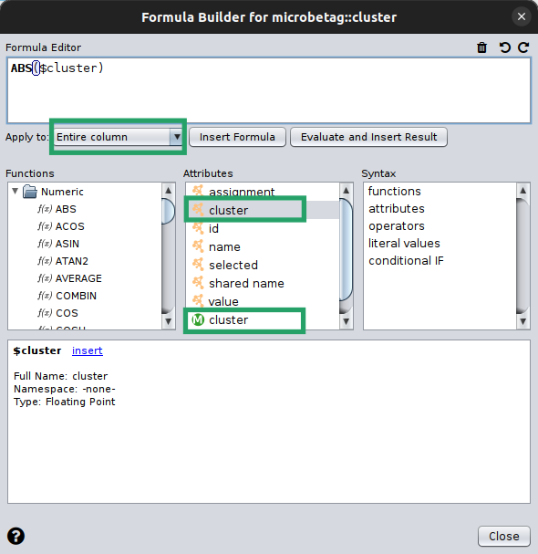
Make sure you apply the function to the whole column!
In this example, you may see that it seems there are two cluster columns, yet they look different! One has the Cytoscape logo on its left, while the other has an M. This is because the new column we created has a different namespace than the rest of the columns on the Node table. If it was not for this, Cytoscape would not allow us to have two columns with the same name!
Our new microbetag::cluster column is now ready, and we are good to go with the next steps! :rocket:
And now, we can load the table with the clusters, by first moving to the network with the FAPROTAX and
the phenDB-like annotations
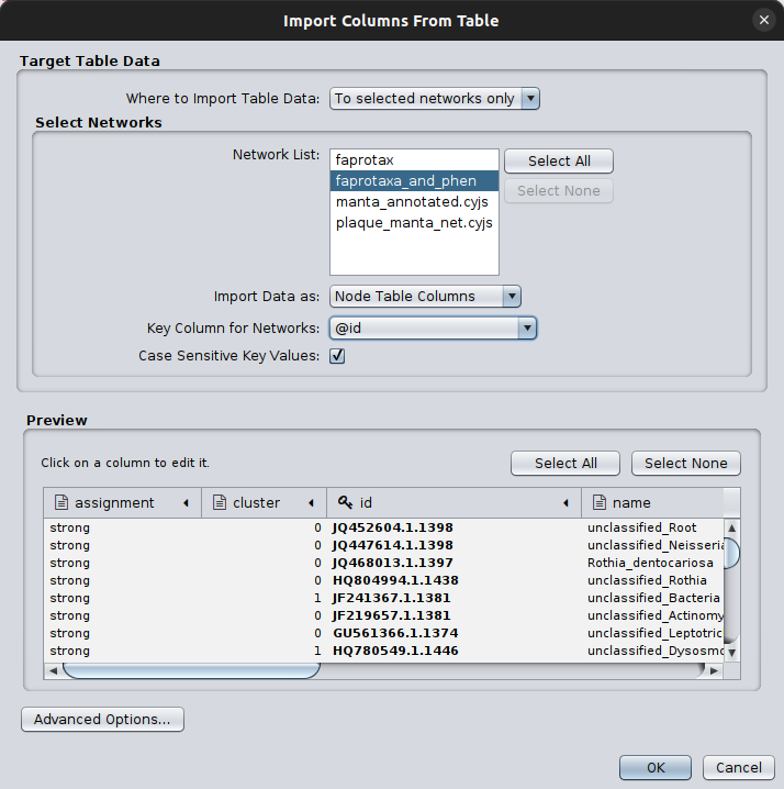
and clicking on the Import Table From File... button.
After selecting the manta_annotated.node.csv, we had to specify:
in which of the open network collections to add the table; in our case we had named this
faprotax_and_phenwhich column to use as a key to map on our network (
@id):
Now, we have all required elements of the nodes’ annotation!
We have both FAPROTAX and phenDB annotations, and we also have clusters!
Therefore, after renaming the cluster column to microbetag::cluster, we are good to go
with the enrichment analysis test!
Hint
Here is a link on how to add data on Cytoscape from spreadsheet tables.